

Memoization!
The name is largely a marketing construct. Here is the
inventor of the term, Richard Bellman, on how it came about:
"I spent the Fall quarter (of 1950) at RAND.
My first task was to find a name
for multistage decision processes.
An interesting question is, Where did the
name, dynamic programming, come from?
The 1950s were not good years for
mathematical research.
We had a very interesting gentleman in Washington named Wilson.
He was Secretary of Defense,
and he actually had a pathological fear
and hatred of the word research.
I'm not using the term lightly; I'm using it precisely.
His face would suffuse, he would turn red,
and he would get violent
if people used the term research in his presence.
You can imagine how he felt,
then, about the term mathematical.
The RAND Corporation was employed by the Air
Force, and the Air Force had Wilson as its boss, essentially.
Hence, I felt I had to do something to shield Wilson
and the Air Force from the fact that I was
really doing mathematics inside the RAND Corporation.
What title, what name,
could I choose? In the first place I was
interested in planning, in decision making, in thinking.
But planning, is not a good word for various reasons.
I decided therefore to use the word "programming".
I wanted to get across the
idea that this was dynamic,
this was multistage, this was time-varying.
I thought, let's kill two birds with one stone.
Let's take a word that has an
absolutely precise meaning, namely dynamic,
in the classical physical sense.
It also has a very interesting property as an adjective,
and that it's impossible
to use the word dynamic in a pejorative sense.
Try thinking of some combination
that will possibly give it a pejorative meaning.
It's impossible.
Thus, I thought dynamic programming was a good name.
It was something not even a
Congressman could object to.
So I used it as an umbrella for my activities."
(Source:
https://en.wikipedia.org/wiki/Dynamic_programming#History)
Note that Bellman's claim that "dynamic" can be use
pejoratively is surely false: most people would not favor
"dynamic ethnic cleansing"!
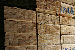
Nothing special here about steel rods: the algorithm applies to
any good that can be sub-divided, but only in multiples of some
unit, like lumber, or meat, or cloth.
Keeps calculating the same cuts again and again, much like
naive, recursive Fibonacci.
Running time is exponential in n. Why?
Our textbook gives us the equation:
This is equivalent to:
T(n) = 1 + T(n - 1) + T(n - 2) + ... T(1)
For n = 1, there are 20 ways to solve the
problem.
For n = 2, there are 21 ways to solve the
problem.
For n = 3, there are 22 ways to solve the
problem.
Each additional foot of rod gives us 2 * (previous number
of ways of solving problem), since we have all the previous
solutions, either with a cut of one foot for the new
extension, or without a cut there. (Similar to why each row
of Pascal's triangle gives us the next power of two.)

So, we have the series:
2n - 1 + 2n - 2 + 2n -
3... + 20 + 1
And this equals 2n. Why?
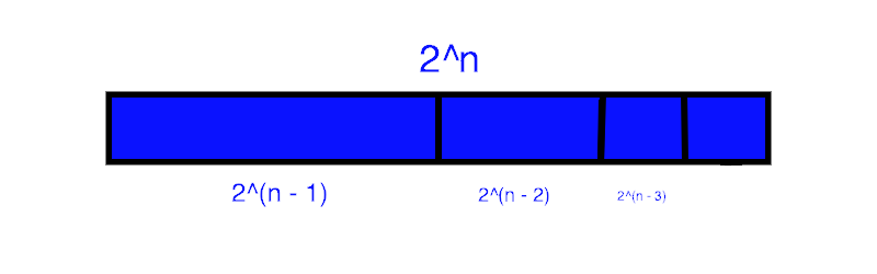
Example: 24 = 23 +
22 + 21 + 20 + 1
Or, 16 = 8 + 4 + 2 + 1 + 1
Much like we did with the naive,
recursive Fibonacci,
we can "memoize" the recursive rod-cutting algorithm and
achieve huge time savings.
That is an efficient top-down approach. But we can also do
a bottom-up approach, which will have the same run-time
order but may be slightly faster due to fewer function
calls. (The algorithm uses an additional loop instead of
recursion to do its work.)

The above is the Fibonacci sub-problem graph for fib(5). As
you can see, F5 must solve F4 and
F3. But F4 must also solve
F3. It also must solve F2, which
F3 must solve as well. And so on.
This is the sort of graph we want to see if dynamic
programming is going to be a good approach: a recursive
solution involves repeatedly solving the same problems.
This is quite different than, say, a parser, where the code
sub-problems are very unlikely to be the same chunks of
code again and again, unless we are parsing the code of a
very bad programmer who doesn't understand functions!
In this section, we see how to record the solution we arrived at, rather than simply return the optimal revenue possible. The owner of Serling Enterprises will surely be much more pleased with this code than the earlier versions.
In the console below, type or paste:
                !git clone https://gist.github.com/80d2a774f08f686f675f8a9254570da0.git


                cd 80d2a774f08f686f675f8a9254570da0


                from dynamic_programming import *
Now let's run our ext_bottom_up_cut_rod() code.
(Link to full source code below.)
Type or paste:
                p4


                (revs, cuts, max_rev) = ext_bottom_up_cut_rod(p4, 4)
You can explore more, by designing your own price
arrays! Just type in:
my_name = [x, y, z...]
where 'my_name' is whatever name you want to give your
price array, and x, y, z, etc. are the prices for a cut
of length 1, 2, 3, etc.

There are many ways to parenthesize a series of matrix
multiplications. For instance, if we are parenthesizing
A1 * A2 * A3 * A4,
we could parenthesize this in the following ways:
(A1 (A2 (A3 A4)))
(A1 ((A2 A3) A4))
((A1 A2) (A3 A4))
((A1 (A2 A3)) A4)
(((A1 A2) A3) A4)
Which way we choose to do so can make a huge difference in
run-time!
Why is this different than rod cutting? Think about this for a moment, and see if you can determine why the problems are not the same.
In rod cutting, a cut of 4-2-2 is the same cut as a
cut of 2-2-4, and the same as a cut of 2-4-2.
That is not at all the case for matrix parenthesization.
The number of solutions is exponential in n, thus brute-force is a bad technique for solving this problem.
For any place at level n where we place
parentheses, we must have optimal parentheses
at level n + 1.
Otherwise, we could substitute
in the optimal n + 1
level parentheses, and level n would be better!
Cut-and-paste proof.
If we know the optimal place to split A1...
An (call it k), then the optimal solution is
that split, plus the optimal solution for A1...
Ak and the optimal solution for
Ak+1... An. Since we don't know k, we
try each possible k in turn, compute the optimal
sub-problem for each such split, and see which pair of
optimal sub-problems yields the optimal (minimum, in this
case) total.
"For example, if we have four matrices ABCD, we compute the
cost required to find each of (A)(BCD), (AB)(CD), and
(ABC)(D), making recursive calls to find the minimum cost
to compute ABC, AB, CD, and BCD. We then choose the best
one."
(https://en.wikipedia.org/wiki/Matrix_chain_multiplication)
An easy way to understand this:
Let's say we need to get from class at NYU Tandon to a
ballgame at Yankee Stadium in the Bronx as fast as
possible. If we choose Grand Central Station as the optimal
high-level split, we must also choose the optimal ways to
get from NYU to Grand Central, and from Grand Central to
Yankee Stadium. It won't do to choose Grand Central, and
then walk from NYU to Grand Central, and CitiBike from
Grand Central to Yankee Stadium: there are faster ways to
do each sub-problem!
CLRS does not offer a recursive version here (they do later in the chapter); they go straight to the bottom-up approach of storing each lowest-level result in a table, avoiding recomputation, and then combine those lower-level results into higher-level ones. The indexing here is very tricky and hard to follow in one's head, but it is worth trying to trace out what is going on by following the code. I have as usual included some print statements to help.
Finally, we use the results computed in step 3 to actually provide the optimal solution, by actually determing where the parentheses go.
Here is the code from our textbook, implemented in Python, runnning on the example where A1 is 10 x 100, A2 is 100 x 5, and A3 is 5 x 50:
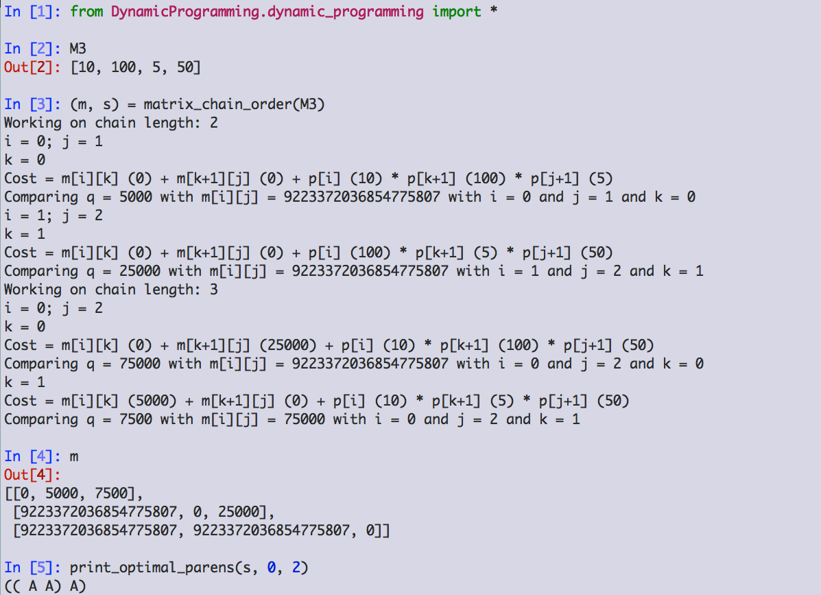
The structure of m:
| 0 | 5000 | 7500 |
| ∞ | 0 | 25000 |
| ∞ | ∞ | 0 |
We can memoize the recursive version and change its run time from Ω(2n) to O(n3).
A problem exhibits optimal substructure if an optimal solution to the problem contains within it optimal solutions to subproblems.
The problem space must be "small," in that a recursive algorithm visits the same sub-problems again and again, rather than continually generating new subproblems. The recursive Fibonacci is an excellent example of this!
Storing our choices in a table as we make them allows quick and simple reconstruction of the optimal solution.
As mentioned above, recursion with memoization is often a viable alternative to the bottom-up approach. Which to choose depends on several factors, one of which being that a recursive approach is often easier to understand. If our algorithm is going to handle small data sets, or not run very often, a recursive approach with memoization may be the right answer.
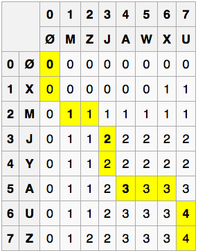
'Let X be "XMJYAUZ" and Y be "MZJAWXU".
The longest common subsequence between X and Y is "MJAU".'
(https://en.wikipedia.org/wiki/Longest_common_subsequence_problem)
Brute force solution runs in exponential time: not so good!
But the problem has an optimal substructure:
X = gregorsamsa
Y = reginaldblack
LCS: regaa
Our match on the last 'a' is at position X11 and
Y11. The previous result string ('rega') must have been
the LCS before X11 and Y11:
otherwise, we could substitute in that actual LCS
for 'rega' and have a longer overall LCS.
Caution: here some sub-problems are ruled out! If Xi and Yj are different, we consider the sub-problems of finding the LCS for Xi and Yj - 1 and for Xi - 1 and Yj, but not for Xi and Yj. Why not? Well, if they aren't equal, they can't be the endpoint of an LCS.
The solution here proceeds much like the earlier ones: find an LCS in a bottom-up fashion, using tables to store intermediate results and information for reconstructing the optimal solution.
We could eliminate a table here, reduce aymptotic
run-time a bit there. But is the code more confusing?
Do we lose an ability (reconstructing the solution) we
might actually need later?
An important principle: Don't optimize unless it is
needed!
![]()
If a binary search tree is optimally construted, then both its left and right sub-trees must be optimally constructed. The usual "cut-and-paste" argument applies.
As usual, this is straightforward, but too slow.
Very much like the matrix-chain-order code. Working code coming soon!
| i | 0 | 1 | 2 | 3 | 4 | 5 |
|---|---|---|---|---|---|---|
| pi | .05 | .05 | .25 | .05 | .05 | |
| qi | .05 | .15 | .05 | .05 | .05 | .20 |