Design and Analysis of Algorithms: Graph Algorithms

Seven Bridges of Königsberg

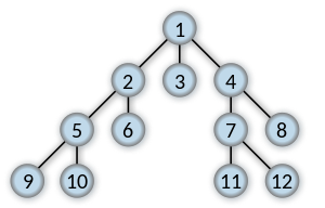
Can one walk the city crossing every bridge once and only once?

Euler answered "No." Why?
View the land as vertices. The bridges are edges. There is an Eulerian walk on a graph only if it is connected and has either zero or two edges of odd degree.

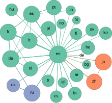
Graph theory was born to solve a problem of movement in space.

But it is also used for:

Task management
Tournament design
Social networks
Map coloring
Voting theory
Cellular telephone networks
Words in a dictionary

Elements:

Walks: Any wandering about from vertex to vertext following edges.
Paths: A walk with no repetition of vertices or edges.
Cycles: Got back to where we were.
Trees: Connected graphs with no cycles.
Forests: Unconnected trees.
Tournaments

Representations of graphs

There are two standard representations:

Adjancency lists
Adjancency matrices

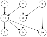
Consider the following graph:

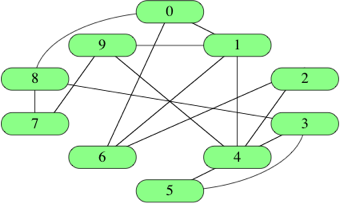
Following our text, we will prefer adjancency lists. But, as CLRS point out, in an especially dense graph, or when we need to detect an edge quickly, we might prefer a matrix.

Here are the two different representations of this graph:

Adjacency list:

Adjacency matrix:

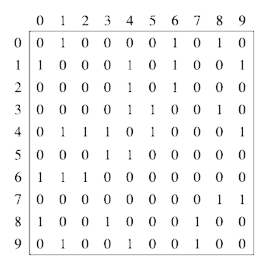
For the adjancency matrix:

Trade-offs

Adjacency list is generally smaller and at worst as large as adjacency matrix. We use it for sparse graphs, where E is singificantly less than V².
Adjacency matrix is simpler. It also allows quicker search for whether some specific edge is present or not.

Both forms can be used to represent directed, undirected, and weighted graphs.
For weighted graphs, we can store 0 or the weight in the matrix instead of just 0 or 1. For the list, we store a tuple (vertex, weight) in the adjancency list of a vertex.
For directed graphs, in a list, i, say, would have an entry for j, but j would not for i. In a matrix, m[i][j] would be 1, but m[j][i] would be 0.

Representing attributes

For pseudo-code, we just represent attribute f of edge (u, v) as (u, v).f. (f might represent the edge already having been visited, for instance.)

In a real program, there are many, many ways to store additional information. How to best do this will very much depend on your application. I have found this can work:

Create a class node.
node has an instance variable adj_list.
Anything you want to put in a graph should sub-class node.
Voila! You can store any attributes whatsoever with each node.

Breadth-first search

We assume a source vertex s.
We then find every vertex at distance 1 from the source. (Connected by a direct edge.)
Then we process those vertices, finding every vertex at distance 2 from the source vertex.
We continue in the same fashion until we run out of vertices.

Coloring vertices:
Vertices start out "white."
They are colored gray when they are discovered.
They are colored black when all of their adjacent vertices have been discovered.

Analysis

After initialization, BFS never whitens a vertex. So each will go on and off the queue at most once. So queue time is O(V).
The adjacency list for each vertex is scanned once, when the vertex is dequeued. The length of all adjacency lists is the number of edges, E. So this runs in O(E).
The overhead for initialization is O(V).
Thus, we get a running time for BFS of O(V + E).

Shortest paths

Breadth-first search computes shortest path distances.

Lemma 22.1
For any edge (u, v) ∈ E,
δ(s, v) ≤ δ(s, u) + 1

Depth-first search

This search goes as "deep" as it can before it ventures back up the graph to explore other nodes nearer the source.

Coloring vertices:
Vertices start out "white."
They are colored gray when they are discovered.
They are colored black when they are "finished," meaning when all of the nodes on their adjacency list have been completely explored.

Properties of depth-first search

Running time: O(V + E)

Classification of edges

Types of edges:

Tree edges:
Edges of the depth-first forest G_π. Edge (u, v) is a tree edge if v was first discovered by exploring edge (u, v).
Back edges:
An edge (u, v) that connects u to an ancestor v.
Forward edges:
Non-tree edge (u, v) that connects u to an descendant v.
Cross edges:
All other edges.

In DFS, when we first explore (u, v) the color of v tells us:

WHITE: This is a tree edge.
GRAY: This is a back edge.
BLACK: This is a forward edge or cross edge.

Topological sort

Can only be performed on directed acyclical graphs (DAGs). The sort makes no sense on undirected graphs or cyclical graphs.

Property: If G contains an edge (u, v), then u appears before v in the topological ordering.

Our book's topological sort algorithm is somewhat weird:
TOPOLOGICAL-SORT(G)

call DFS(G) to compute finishing times v.f for each vertex v.
as each vertex is finished, insert it into the front of a linked list
return the linked list of vertices.

Strongly connected components

These are components of directed graphs that can each be reached from the other.
Many advanced graph algorithms rely on de-composing a graph into strongly directed components, and then processing those, and then combining the results: divide-and-conquer!

Algorithm:

Call DFS(G) to compute finish times for each vertex.
Compute

Source Code

Python
Ruby

For Further Study

Graph (abstract data type)

Credits

Graphics of list versus matrix representations: https://www.khanacademy.org/computing/computer-science/algorithms/graph-representation/a/representing-graphs