
An algorithm is a finite sequence of precise instructions for performing a computation or for solving a problem.
Algorithm for finding the maximum (largest) value in a finite sequence of integers: Solution Steps:
Properties of an Algorithm
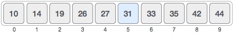
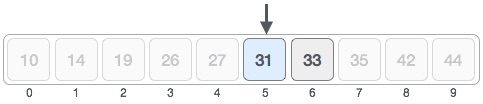
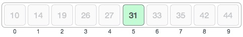
The problem of locating an element in an ordered list occurs in many contexts. For instance, a program that checks the spelling of words searches for them in a dictionary, which is just an ordered list of words. Problems of this kind are called searching problems.
procedure linear search(x: integer,
a1, a2, .
. . , an: distinct integers)
i := 1
while (i ≤ n
and x != a[i] )
i = i + 1
if i ≤ n then
location := i
else location := 0
return location
{location is the subscript of
the term that equals x,
or is 0 if x is not found}
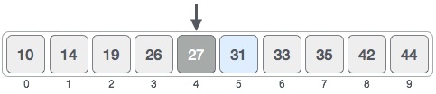
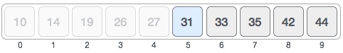
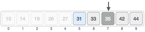
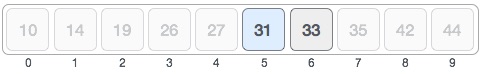
This algorithm can be used when
the list has terms occurring in
order of increasing size (for instance:
if the terms are numbers,
they are listed from smallest to largest;
if they are words, they
are listed in lexicographic, or alphabetic,
order). This second
searching algorithm is called the binary search algorithm.

Psuedocode
            procedure bubblesort(a1, a2, . . . , an: real numbers n ≥ 2)
            for ( i := 1 to n-1)
            for ( j to n-1)
            if a  j > aj+1 then interchange aj and aj+1

            {a1, . . . ,a n is in increasing order}
procedure
insertionsort(a1, a2, .
. . , an: real numbers n ≥ 2)
for ( j := 2 to n)
i := 1
while a j >
ai
i := i+1
m := aj
for k := 0 to j − i − 1
aj−k
:= aj
−k
− 1
ai := m
{a1, . . . ,
an}
Algorithms that make what seems to be the best
choice at each step are called greedy algorithms.
Greedy Change-Making Algorithm
procedure
change(c1, c2, .
. . , cn: value of denominations
where c1 > c2 > .
. . , cn : n is a positive
integer)
for ( i := 1 to r)
di := 0 {di
counts the number of denominations ci
used
while n ≥
ci
di := di +
1 {add a coin of denomination ci }
n := n - ci
di is the number of coins of
denominations in ci in change for
i = 1, 2, 3
LEMMA 1
If n is a positive integer, then n cents in change using quarters, dimes, nickels, and pennies using the fewest coins possible has at most two dimes, at most one nickel, at most four pennies, and cannot have two dimes and a nickel. The amount of change in dimes, nickels, and pennies cannot exceed 24 cents.
THEOREM 1
The greedy algorithm produces change using the
fewest coins possible.
Greedy Algorithm for Scheduling Talks
procedure
schedule(s1 ≤
s2 ≤ .
. . , sn: start time of talks
e1 ≤ e2 ≤ .
. . , en : n ending times
of talks)
sort talks by finish time and reorder so that e1 ≤
e2 ≤ . . , en
S := 0
for ( i := 1 to n)
if talk j is compatible with S
S := S &union; {talk j}
return S{ S is the set of talks produced}
1. c; 2. a; 3. b; 4. b; 5. a; 6. d; 7. c; 8. b; 9. a;
DEFINITION
Let f and g be functions
from the set of integers
or the set of real numbers to the set
of real numbers.We say that
f(x) is O(g(x)) if
there are constants C and
k such that |f(x)|
≤ C|g(x)|whenever
x > k.
(This is read as "f(x)
is big-oh of g(x).")
Example 1
Show that
f(x) = 7x2 is
O(x3).
Take C = 1 and k
= 7 as witnesses to establish
that 7x2
is O(x3).
When x > 7,
7x2 < x3.
Consequently, we can take
C= 1 and k = 7 as
witnesses to establish the
relationship 7x2 is
O(x3).
Alternatively, when x
> 1, we have 7x2 <
7x3,
so that C = 7
and k = 1 are also
witnesses to the relationship
7x2 is O(x3).
THEOREM 1
Let f(x) =
an
xn +
an −
1xn
− 1 +...+
ax + a,
where a0,
a1...
an − 1,
an are real numbers.
Let f(x) =
anxn +
an −
1xn −1
+...+ ax + a,
where a0,
a1...
an − 1,
an are real numbers.
Then f(x) is
O(xn).
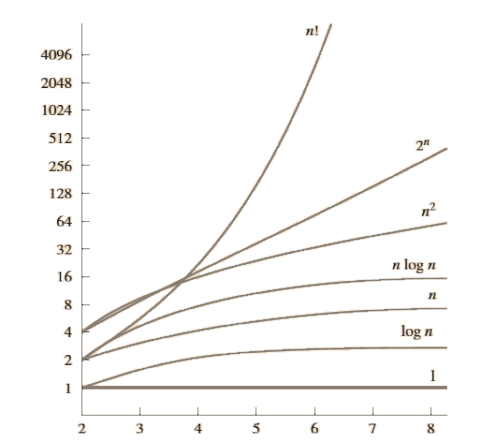
A Display of the Growth
of Functions Commonly Used in Big-O
Estimates.
THEOREM 2
Suppose that f1(x) is
O(g1(x)) and that
f2(x)
is O(g2(x)).
Then (f1
+ f2)
(x) is O
(max(|g1
(x)|, |g2(x)|)).
COROLLARY 1
Suppose that f1(x) and
f2(x)
are both O(g(x)).
Then (f1 +
f2)(x) is
O(g(x)).
THEOREM 3
Suppose that f1(x)
is O(g1(x))
and f2(x)
is O(g2(x)).
Then (f1f2)
(x) is
O(g1(x)g2(x)).
DEFINITION 2
Let f and g be
functions from the set of integers
or the set of real numbers to
the set of real numbers.We say that
f(x) is Ω;
(g(x) if there are positive constants
C and k such that |f(x)| ≥
C|g(x)|
whenever x > k.
(This is read as "f(x
is big-Omega of g(x.")
Example: Show that
f(x) = x3 is
Ω(7x2).
DEFINITION 3
Let f and g be
functions from the set of integers
or the set of real numbers to
the set of real numbers.We say that
f(x) is θ(g(x))
if f(x) is O(g(x)
and f(x) is Ω(g(x)).
When f(x)is
Θ(g(x)) we say that f
is big-Theta of g(x),
that f(x) is of order g(x),
and that f(x) and
g(x) are of the same order.
Example: Show that 3x2+ 8x
log x is Θ(x2).
THEOREM 4
Let f(x) =
anxn +
an-1xn −
1
+...+ a1
+ a0, where a0,
a1, . . . ,
an are real numbers
with an ≠ 0.
an −
1 x n - 1
+ . . . + a1x
+ a0, where a0,
a1, . . . ,
an are real numbers
with an ≠ 0.
Then f(x) is of
order xn.
Algorithms class lecture on the growth of functions.
1. b; 2. b; 3. a; 4. a; 5. a; 6. b;
An analysis of the time required
to solve a problem of a particular
size involves the time complexity
of the algorithm.The time complexity of
an algorithm can be expressed
in terms of the number of operations
used by the algorithm when
the input has a particular size.
In most of the cases we consider
the worst-case time complexity of an
algorithm. This provides an upper
bound on the number of operations an
algorithm uses to solve a problem
with input of a particular size.
Complexity Analysis of Some Algorithms
Example:
Describe the time
complexity of an Algorithm for finding
the maximum element in a finite set of integers.
An analysis of the time required to
solve a problem of a particular
size involves the time
complexity of the algorithm.
The time complexity of
an algorithm can be expressed in
terms of the number of operations
used by the algorithm when the
input has a particular size.
In most of the cases we consider the
worst-case time complexity of an
algorithm. This provides an upper bound
on the number of operations an
algorithm uses to solve a problem
with input of a particular size.
Example:
Describe the
time complexity of an Algorithm
for finding the maximum element
in a finite set of integers.
The definition of the product
of two matrices can be expressed as an
algorithm for computing the
product of two matrices. Suppose that
C = [cij] is the
m ✕ n matrix that is the
product of the m ✕ k
matrix A = [aij]
and the k ✕ n matrix
B = [bij ].
The definition of the product of two matrices can
be expressed as an
algorithm for computing the product of
two matrices. Suppose that
C = [cij]
is the m ✕ n matrix that is the
product of the m ✕ k
matrix A = [aij]
and the k ✕ n
matrix B = [bij ].
Pseudocode Matrix Multiplication
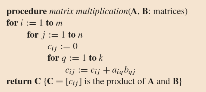
Complexity Calculation How many additions of integers and multiplications of integers are used by the matrix multiplication algorithm to multiply two n * n matrices.
Algorithm Paradigms is a general
approach based on a particular concept
that can be used to construct algorithms
for solving a variety of problems.
Greedy Algorithm, Divide-and-Conquer Algorithm,
Brute Force Algorithm, and Probabilistic
Algorithm are algorithm paradigms.
Example:
Brute Force Algorithms
A brute-force algorithm is solved in the most
straightforward manner,
without taking advantage of any ideas
that can make the algorithm more efficient.
Construct a brute-force algorithm for finding
the closest pair of
points in a set of n points in the
plane and provide a worst-case
estimate of the number of arithmetic operations.
Pseudocode for Brute-Force Closest Point Algorithm
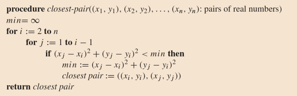
Complexity of the Algorithm
The algorithm loops through
n(n - 1)/2 pairs of
points, computes the value
(xj -
xi)2+
(yj -
yi)2and
compares it with the minimum, etc.
So, the algorithm uses
Θ(n2)
The algorithm loops through n(n − 1)/2
pairs of points, computes the value
(xj −
xi)2 +
(yj −
yi)2 and
compares it with the minimum, etc. So, the algorithm uses
Θ(n2)
arithmetic and comparison operations.
| Commonly Used Terminology for the Complexity of Algorithms. | |
|---|---|
| Complexity | Terminology |
| Θ(1) | Constant Complexity |
| Θ(log n) | Logarithmic Complexity |
| Θ(n) | Linear Complexity |
| Θ(n log n) | Linearithmic complexity |
| Θ(nb) | Polynomial complexity |
| Θ(bn) where b >1 | Exponential Complexity |
| Θ(n!) | Factorial Complexity |
Tractable problem: a problem
for which there is a worst-case
polynomial-time algorithm that solves it
Intractable problem: a
problem for which no worst-case
polynomial-time algorithm exists for solving it
Solvable problem: a problem
that can be solved by an algorithm
Unsolvable problem: a problem
that cannot be solved by an
algorithm
1. b; 2. b; 3. d; 4. b; 5. a; 6. a;