

It is important to recognize that we have been dealing with a family of problems and solutions to those problems:
We have an optimization problem.
At each step of the algorithm, we have to make a choice, e.g.,
cut the rod here, or cut it there.
Sometimes, we need to calculate the result of all possible
choices.
But sometimes, we can do much better than either of those
choices. Sometimes, we don't need to consider the global
situation at all: we can simply make the best choice among the
options provided by the local problem we face, and then
continue that procedure for all subsequent local problems.
An algorithm that operates in such a fashion is a greedy
algorithm. (The name comes from the idea that the
algorithm greedily grabs the best choice available to it right
away.)
Clearly, not all problems can be solved by greedy algorithms.
Consider this simple shortest path problem:
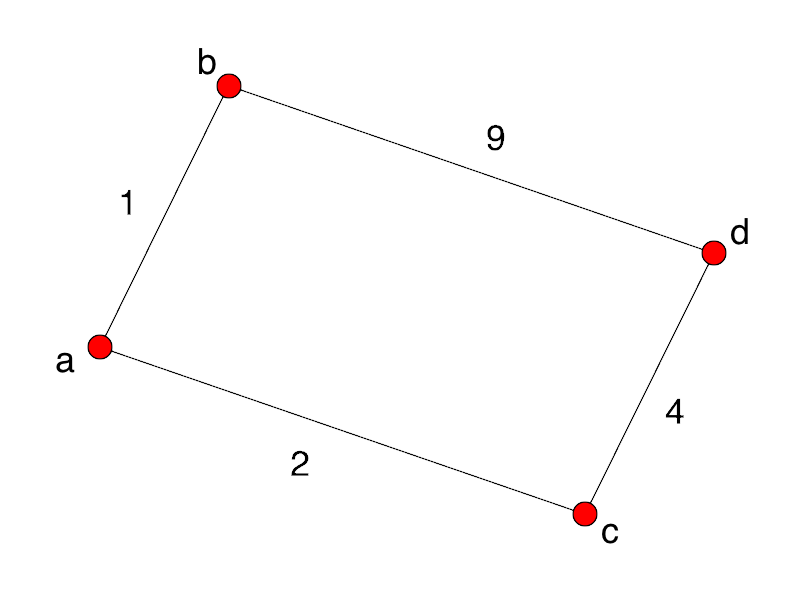
A greedy algorithm choosing the shortest path from a to d will
wrongly head to b first, rather than to c.
Suppose we need to schedule a lecture hall with the goal of
maximizing the number of lectures it can hold, given the
constraint that no lectures can share the space.
We have the activities sorted in order of increasing finish
time:
f1 ≤ f2 ≤ f3
≤ ... ≤ fn - 1 ≤ fn.
We might have the following set of activities:
| i | 1 | 2 | 3 | 4 | 5 | 6 | 7 | 8 | 9 | 10 | 11 |
|---|---|---|---|---|---|---|---|---|---|---|---|
| si | 1 | 3 | 0 | 5 | 3 | 5 | 6 | 8 | 8 | 2 | 12 |
| fi | 4 | 5 | 6 | 7 | 9 | 9 | 10 | 11 | 12 | 14 | 16 |
We have several sets of mutually compatible lectures, e.g.:
{a3,
a9,
a11}
However, this set is larger:
{a1,
a4,
a8,
a11}
How do we find the maximum subset of lectures we can
schedule?
It is easy to see that the problem exhibits optimal
substructure. If the optimal solution includes a
lecture from 4 to 6, then we have the sub-problems of
scheduling lectures that end by 4, and lectures that start
at 6 or after. Obviously, we must solve each of those
sub-problems in an optimal way, or our solution will not be
optimal! (Think of our problem of traveling from MetroTech
Center to Yankee Stadium via Grand Central.) Our textbook
calls this a "cut-and-paste" argument: we can cut an
optimal set of lectures ending by 4 and paste it into our
supposed optimal solution: if the solution was different
before 4, we have improved it, so it wasn't actually
optimal!
It is straight forward to see that we
can solve this problem with a recursive,
memoized algorithm -- we examine each
possible "cut" of a "middle" lecture, and recursively solve
the start-to-middle problem, and the middle-to-end problem.
Or we could use a bottom-up dynamic programming algorithm,
developed from the recursive solution in the same way we
saw in our last lecture.
But we can solve this problem much more efficiently. At
each step in solving it, we can make a completely local
choice: what activity (still possible) finishes earliest?
Since we have sorted the activities in order of increasing
finish time, we simply choose a1, since
it is guaranteed to finish at least tied for first.
The proof that this will give us a maximal set of
activities is trivial: Let us suppose aj
is the activity in some set that finishes first, but that
there is a maximal subset Ak
that does not include
aj. We simply remove the first element of
Ak and substitute in aj. This
is guaranteed to be a compatible set of activities, since
aj finishes first, and it will be
maximal, since it is the same size as Ak. (Note
that the textbook offers us an example of such sets on page
415.)
The algorithm is straightforward:
find the first compatible activity, then call
the algorithm again with the rest of the activity list.
One trick worth noting:
the authors put a dummy activity in the
first position of the list, so that there
is no special first call of the function.
There is a design pattern here: oftentimes, it is
better to modify a data structure than to do
special coding for end cases.
            Recursive-Activity-Selector(s, f, k, n)
                m = k + 1
                while m ≤ n and s[m] < f[k]
                    m = m + 1
                if m ≤ n
                    // + here is set union!
                    return a[m] + Recursive-Activity-Selector(s, f, m, n)
                else
                    return NIL
As usual, it is fairly simple to transform the recursive algorithm into an iterative version. The authors discuss tail recursion in this section: let's review what this is.
            Greedy-Activity-Selector(s, f)
                n = s.length
                A = {a[1]}
                k = 1
                for m = 2 to n
                    if s[m] > f[k]
                        A = A + {a[m]} // + is set union!
                        k = m
                return A
In the console below, type or paste:
                          !git clone https://gist.github.com/bb22ea72d8b15fa965d2f50e6798ae50.git


                          cd bb22ea72d8b15fa965d2f50e6798ae50


                          from greedy_algorithms import *


                          print("start: ", start, "\nfinish: ", finish)


                          greedy_activity_selector(start, finish)

For a greedy algorithm to work, the optimal choice must not
depend upon any sub-problems or any future choices.
To prove that a greedy choice will be appropriate for some
problem, we typically examine an optimal solution, and then
show that substituting in a greedy choice will also yield an
optimal solution.
This is simpler then for dynamic programming problems: all we need to do is show that a greedy choice combined with an optimal solution to the sub problem of the rest of the data gives us an optimal solution to the original problem. We use induction to show that making the greedy choice at every step produces an optimal solution.
Two knapsack problems:
The latter can be solved with a greedy algorithm, the former cannot.

Hoffman coding is away of compressing data that consists of
characters buy creating short binary representations for the
characters that occur most frequently in the data, and using longer
representations for characters that occur less frequently.
Prefix codes are coding schemes in which no codeword
is a prefix of a different codeword.
This makes decoding easier -- no lookahead.
(else and else-if)
It means that we never hit two letters on the same path
down the tree!
| a | b | c | d | e | f | |
|---|---|---|---|---|---|---|
| Frequency (in 1000s) | 45 | 13 | 12 | 16 | 9 | 5 |
| Codeword | 0 | 101 | 100 | 111 | 1101 | 1100 |
We build a binary tree from the bottom-up, starting with the
two least-frequent characters, and building up from there. This
ensures the least-frequent characters have the longest codes.
Consider the phrase "Mississippi River".
This is 136 bits in 8-bit ASCII encoding.
Here is the Huffman coding for it:
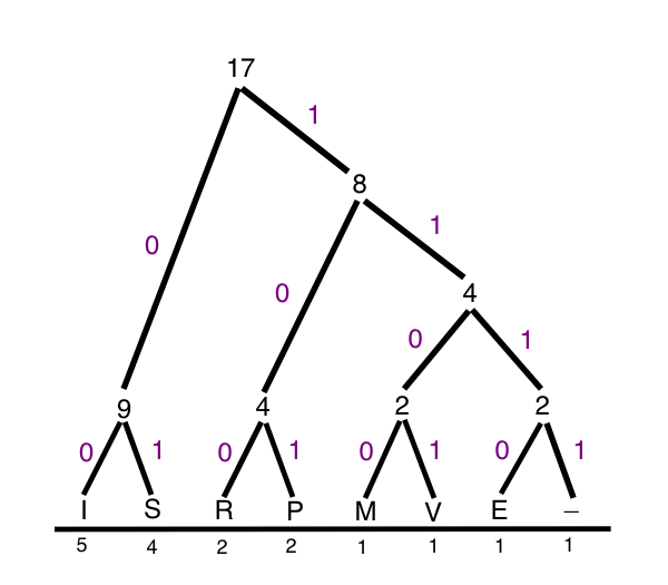
I = 00
S = 01
P = 100
R - 101
M = 1100
V = 1101
E = 1110
_ = 1111
The final string:
110000010100010100100100001111101001101101
Try parsing it, and convince yourself that there is
only one possible interpretation of it. That is what
the prefix coding buys us.
We begin operating on an alphabet Σ. At each step,
we create a new alphabet, Σ', with two symbols of
Σ replaced by a new "meta-symbol".
Base case: For an alphabet of two symbols, the
algorithm outputs 0 for one of them, and 1 for the
other. And that is clearly optimal! (An alphabet of
size 1 is a non-problem!)
Inductive step: Assume the algorithm is correct
for input of size n - 1.
At each step in the algorithm, we replace the two least
frequent remaining symbols a and b with a
new symbol ab, whose probability is the sum of
the probabilities of a and b.
We always want the lowest frequency symbols to have the
longest encoding length.
Any choice among symbols at the lowest frequency will
be fine, since they all have equally low frequency. So
we can pair any of those lowest frequency symbols as we
wish.
Now assume that there is an encoding Σ'' that is
derived from Σ (like Σ') but differs in
choosing to combine x and y into a
xy. But since we made the greedy choice,
xy can be at best tied with ab meaning
Σ'' is at best another optimal encoding, and our
encoding Σ' is optimal after all.

Consider the following graph, where the edges represent
roads and the vertices towns:
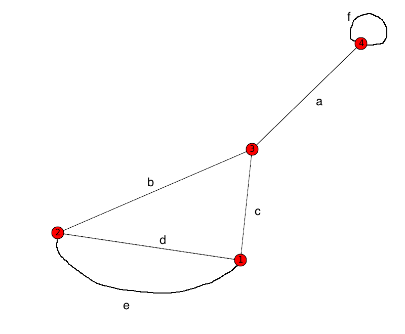
If we want to build a set of roads that are only built
if there is no other route between towns, what sets are
possible?
Notice:
Now look at the following vector space in
ℝ3:
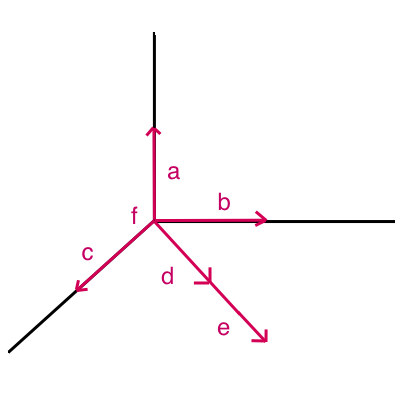
(f is the vector 0, 0, 0.)
What sets of linearly independent vectors are possible?
Notice:
You live in a small town with 3 women and 5 men who are
single but might be married off. There is a town
matchmaker who makes money by arranging marriages, and
so he wants to arrange as many as possible.
In this town, it's "ladies' choice," and the women are
numbered 1-3, and the men are a-f.

What sets of matches are possible?
Notice:
We are looking at general
conditions for independence
of choices. All three situations turn out to be
surprisingly similar. They can all
be modeled using matroids.
We have a matroid when the following independence
conditions are satisfied:
A matroid consists of (S, I), where S is a set, and I
is a set of subsets of S, for which axioms 1-3
above are satisfied.
All three situations described above, the vector space,
the graph, and the matching problem, turn out to be the
same matroid.
(Technically, they are isomorphic matroids.)
A subset in I is a basis for a
matroid if it is a maximal
subset, which here means it is not contained in any
larger subset that is in I.
So in the above examples, the bases are:
{a, b, c} {a, b, d}, {a, b, e} {a, c, d} {a, c, e}
Theorem:
Every basis of a matroid is of the same size.
Proof: Let assume that there are some bases
A and B of a matroid such that |B| < |A|.
Then by the exchange axiom (#3 above),
there is some
element a of A that can be moved
into B, and B
will still be independent.
Therefore, it was not
a maximal independent subset after
all!
Translation into the different matroid realms:
The dimension of a vector space is the
size of any of its bases.
Every spanning tree has the same number of edges.
We are proving things about vector spaces and graphs
simply by examining the axioms of matroids!
This section draws on lectures by Federico Ardila: here and here.
Q: Why do greedy algorithms work on a matroid?
A: Independence!
We often have a problem that can be considered as an instance of finding a maximum (or minimum) weight independent subset in a weighted matroid. Let us look at Kruskal's algorithm.

The surprise here is that we can
simply greedily grab tasks in
order of increasing deadlines, and our algorithm will work.